Page 25 - 2023-ml-lewandowski-stats1e

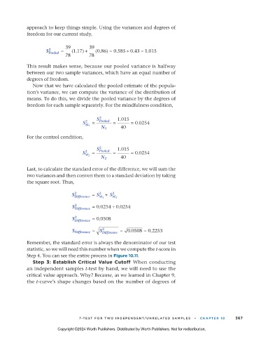
approach to keep things simple. Using the variances and degrees of
freedom for our current study,

39 39
S 2 = (1.17) + (0.86) = 0.585 + 0.43 = 1.015
Pooled
78 78
This result makes sense, because our pooled variance is halfway
between our two sample variances, which have an equal number of
degrees of freedom.
Now that we have calculated the pooled estimate of the popula-
tion’s variance, we can compute the variance of the distribution of
means. To do this, we divide the pooled variance by the degrees of
freedom for each sample separately. For the mindfulness condition,

S 2 1.015
S 2 = Pooled = = 0.0254
M 1 40
N 1
For the control condition,

S 2 1.015
S 2 = Pooled = = 0.0254
M 2 40
N 2
Last, to calculate the standard error of the difference, we will sum the
two variances and then convert them to a standard deviation by taking
the square root. Thus,

2
S 2 Difference = S 2 M 1 + S M 2
2
S Difference = 0.0254 + 0.0254
2
S Difference = 0.0508
= S 2 = 0.0508 = 0.2253
S Difference Difference
Remember, the standard error is always the denominator of our test
statistic, so we will need this number when we compute the t-score in
Step 4. You can see the entire process in Figure 10.11.
Step 3: Establish Critical Value Cutoff When conducting
an independent samples t-test by hand, we will need to use the
critical value approach. Why? Because, as we learned in Chapter 9,
the t-curve’s shape changes based on the number of degrees of

T -TES T F OR TW O INDEPENDENT/UNRELATED S AMPLES • CHAPTER 10 367

Copyright ©2024 Worth Publishers. Distributed by Worth Publishers. Not for redistribution.

11_statsresandlife1e_24717_ch10_343_389.indd 367 29/06/23 5:17 PM