Page 26 - 2023-ml-lewandowski-stats1e

Two
Independent
Samples
2
2
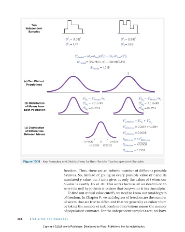
S = (1.08) 2 S = (0.93) 2
2
1
2
2
S = 1.17 S = 0.86
1 2
2
2
S 2 Pooled = (df /df Total )(S ) + (df /df Total )(S )
1
1
2
2
S 2 Pooled = (39/78)(1.17) + (39/78)(0.86)
S 2 Pooled = 1.015
1 2
(a) Two Distinct
Populations
S 2 M = S 2 Pooled /N 1 S 2 M = S 2 Pooled /N 2
2
1
(b) Distribution S 2 M = 1.015/40 S 2 M = 1.015/40
of Means from S 2 1 = 0.0254 S 2 2 = 0.0254
Each Population M M
1
2
S 2 Difference = S 2 M + S 2 M 2
1
(c) Distribution S 2 Difference = 0.0254 + 0.0254
of Differences 2
Between Means S Difference = 0.0508
S Difference = S 2 Difference
–0.4506 0 0.4506
–0.2253 0.2253 S Difference = 0.0508
S Difference = 0.2253

Figure 10.11 Key Formulas and Distributions for the t-Test for Two Independent Samples

freedom. Thus, there are an infinite number of different possible
t-curves. So, instead of giving us every possible value of t and its
associated p-value, our t-table gives us only the values of t when our
p-value is exactly .05 or .01. This works because all we need to do to
reject the null hypothesis is to show that our p-value is less than alpha.
To find our critical value cutoffs, we need to know our total degrees
of freedom. In Chapter 9, we said degrees of freedom are the number
of scores that are free to differ, and that we generally calculate them
by taking the number of independent observations minus the number
of population estimates. For the independent samples t-test, we have

368 S TATIS TI c S F OR R ESEAR c H

Copyright ©2024 Worth Publishers. Distributed by Worth Publishers. Not for redistribution.

11_statsresandlife1e_24717_ch10_343_389.indd 368 29/06/23 5:17 PM