Page 42 - 2023-bfw-Macro-Krugman-Econ-4e

ModULE 1.5
curve. A market with many producers will supply a larger quantity of a good than a
market with a single producer, all other things equal. For example, when the patent
runs out on a profitable pharmaceutical drug, new suppliers can enter the market and
the supply increases.

Changes in Technology When economists talk about “technology,” they mean
all the methods people can use to turn inputs into useful goods and services. In that
sense, the whole complex sequence of activities that turn lumber from harvested and
milled in Canada into the shelves in your closet is technology.
Improvements in technology enable producers to spend less on inputs yet still pro-
duce the same output. When a better technology becomes available, reducing the cost
of production, supply increases, and the supply curve shifts to the right. As we have
already mentioned, improved technology enabled sawmills to keep lumber prices low
for decades, even as worldwide demand grew.
Individual Versus Market Supply Curves
Now that we have introduced the market supply curve, let’s examine how it relates to a
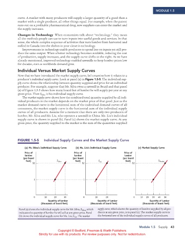
producer’s individual supply curve. Look at panel (a) in Figure 1.5-5. The individual sup-
ply curve shows the relationship between quantity supplied and price for an individual
producer. For example, suppose that Mr. Silva owns a sawmill in Brazil and that panel
(a) of Figure 1.5-5 shows how many board feet of lumber he will supply per year at any
given price. Then S Silva is his individual supply curve.
The market supply curve shows how the combined total quantity supplied by all indi-
vidual producers in the market depends on the market price of that good. Just as the
market demand curve is the horizontal sum of the individual demand curves of all
consumers, the market supply curve is the horizontal sum of the individual supply
curves of all producers. Assume for a moment that there are only two producers of
lumber, Mr. Silva and Ms. Liu, who operates a sawmill in China. Ms. Liu’s individual
supply curve is shown in panel (b). Panel (c) shows the market supply curve. At any
given price, the quantity supplied to the market is the sum of the quantities supplied

FIGURE 1.5-5 Individual Supply Curves and the Market Supply Curve

(a) Mr. Silva’s Individual Supply Curve (b) Ms. Liu’s Individual Supply Curve (c) Market Supply Curve
Price of Price of Price of
lumber lumber lumber
(per board (per board (per board
foot) S Silva foot) S Liu foot) S Market
$2 $2 $2

1 1 1

0 10 20 30 0 10 20 0 10 20 30 40 50
Quantity of lumber Quantity of lumber Quantity of lumber
(thousands of board feet) (thousands of board feet) (thousands of board feet)
Panel (a) shows the individual supply curve for Mr. Silva, S Silva , which supply curve, which shows the quantity of lumber supplied by all pro-
indicates the quantity of lumber he will sell at any given price. Panel ducers at any given price, is in panel (c). The market supply curve is
(b) shows the individual supply curve for Ms. Liu, S . The market the horizontal sum of the individual supply curves of all producers.
Liu

Module 1.5 Supply 43
Copyright © Bedford, Freeman & Worth Publishers.
Strictly for use with its products. For review purposes only. Not for redistribution.

02_APKrugman4e_40932_MacroU01_002_062.indd 43 05/07/22 10:51 AM