Page 38 - 2023-bfw-Macro-Krugman-Econ-4e

ModULE 1.5
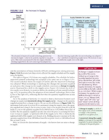
FIGURE 1.5-2 An Increase in Supply

Price of
lumber Supply Schedules for Lumber
(per board foot)
S 1 S 2 Quantity of lumber supplied
$2.00 (billions of board feet)
Price of
Supply curve lumber Before new After new
1.75 before new (per board foot) technology technology
technology
1.50 $2.00 116 139
1.75 115 138
1.25 1.50 112 134
1.25 107 128
1.00 1.00 100 120
Supply curve 0.75 91 109
0.75 after new 0.50 80 96
technology
0.50

0 70 90 110 130 150 170
Quantity of lumber
(billions of board feet)
The adoption of improved sawmill technology generated an the other showing supply after the new technology was adopted
increase in supply — a rise in the quantity supplied at any given (S 2 ) — and their corresponding supply curves. The increase in sup-
price. This event is represented by the two supply schedules — one ply shifts the supply curve to the right.
showing supply before the new technology was adopted (S 1 ),

®
AP ECoN TIP
and the automation of many formerly difficult and dangerous sawing processes. A change in supply is shown
Figure 1.5-2 illustrates how these events affected the supply schedule and the supply by a shift of the curve,
curve for lumber. indicating a change in the
The table in Figure 1.5-2 shows two supply schedules. The schedule for before quantity supplied at every
improved sawmill technology was adopted is the same one as in Figure 1.5-1. price. Remember, left is less
The second schedule shows the supply of lumber after the improved technology and right is more. But looks
was adopted. When technology or anything else changes the quantity supplied can be deceiving. When
at each price, this change in the supply schedule constitutes a change in supply supply decreases, the supply
and is illustrated by a shift in the supply curve. Figure 1.5-2 shows the shift of curve shifts to the left — which
the supply curve from S , its position before the adoption of new sawmill technol- is up, not down. When supply
1
ogy, to S its position after the adoption of new sawmill technology. Notice that increases, the supply curve
2,
S lies to the right of S , reflecting the fact that the quantity supplied rises at any shifts to the right — which is
1
2
given price. down, not up. Always think
As in the analysis of demand, it’s crucial to draw a distinction between such “right” and “left” (not “up”
changes in supply and movements along the supply curve — changes in the quantity and “down”) when shifting
supplied arising from a change in price. We can see this difference in Figure 1.5-3. The supply and demand curves.
movement from point A to point B is a movement along the supply curve: the quan-
tity supplied rises along S due to a rise in price. Here, a rise in price from $1 to $1.50
1
leads to a rise in the quantity supplied from 100 billion to 110.2 billion board feet of A change in supply is a shift of
lumber. But the quantity supplied can also rise when the price is unchanged if there the supply curve, which indicates
a change in the quantity
is an increase in supply — a rightward shift of the supply curve. This is shown by the supplied at any given price.
rightward shift of the supply curve from S to S . Holding the price constant at $1, the
2
1
quantity supplied rises from 100 billion board feet at point A on S to 120 billion board A movement along the supply
1
feet at point C on S . curve is a change in the quantity
2
Next, we discuss the determinants of supply — the factors that can cause a change supplied of a good arising from
in supply. a change in the good’s price.

Module 1.5 Supply 39
Copyright © Bedford, Freeman & Worth Publishers.
Strictly for use with its products. For review purposes only. Not for redistribution.

02_APKrugman4e_40932_MacroU01_002_062.indd 39 05/07/22 10:51 AM