Page 13 - 2023-ml-lewandowski-stats1e

of the difference (3), changes as well. For example, if the 5 becomes a
6, the difference between the numbers changes ( −6 2 = 4). Similarly,
if we vary the 2 and make it a 3, the difference score changes again
( −53 = 2). In other words, when calculating differences, variation in
either number coincides with greater variation in the difference score.
For that reason, when we look at two samples, each sample’s variation
impacts variation in the differences between them.
What that means for our calculation is that we have to add the
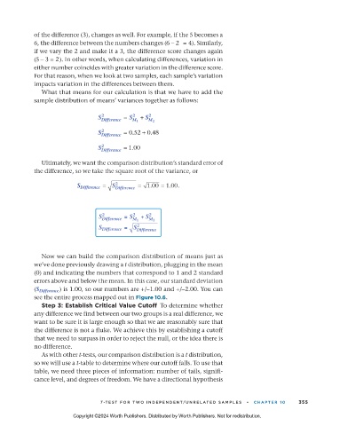
sample distribution of means’ variances together as follows:

2
S 2 Difference = S M 1 + S 2 M 2
S 2 Difference = 0.52 + 0.48

S 2 Difference = 1.00
Ultimately, we want the comparison distribution’s standard error of
the difference, so we take the square root of the variance, or

= S 2 = 1.00 = 1.00.
S Difference Difference

2
S 2 Difference = S 2 M 1 + S M 2
S Difference = S 2 Difference

Now we can build the comparison distribution of means just as
we’ve done previously drawing a t distribution, plugging in the mean
(0) and indicating the numbers that correspond to 1 and 2 standard
errors above and below the mean. In this case, our standard deviation
(S Difference ) is 1.00, so our numbers are + −1.00 and + −2.00. You can
/
/
see the entire process mapped out in Figure 10.6.
Step 3: Establish Critical Value Cutoff To determine whether
any difference we find between our two groups is a real difference, we
want to be sure it is large enough so that we are reasonably sure that
the difference is not a fluke. We achieve this by establishing a cutoff
that we need to surpass in order to reject the null, or the idea there is
no difference.
As with other t-tests, our comparison distribution is a t distribution,
so we will use a t-table to determine where our cutoff falls. To use that
table, we need three pieces of information: number of tails, signifi-
cance level, and degrees of freedom. We have a directional hypothesis

T -TES T F OR TW O INDEPENDENT/UNRELATED S AMPLES • CHAPTER 10 355

Copyright ©2024 Worth Publishers. Distributed by Worth Publishers. Not for redistribution.

11_statsresandlife1e_24717_ch10_343_389.indd 355 29/06/23 5:17 PM