Page 14 - 2023-ml-lewandowski-stats1e

Two
Independent
Samples

2
2
S = SS /df 1 S = SS /df 2
1
1
2
2
2
2
S = 62.22/11 S = 82.00/12
1 2
2
2
S = 5.66 S = 6.83
2
1
2
2
S 2 Pooled = (df /df Total )(S ) + (df /df Total )(S )
1
2
2
1
S 2 Pooled = (11/23)(5.66) + (12/23)(6.83)
S 2 Pooled = 6.27
1 2
(a) Two Distinct
Populations
S 2 M = S 2 Pooled /N 1 S 2 M = S 2 Pooled /N 2
2
1
(b) Distribution S 2 M = 6.27/12 S 2 M = 6.27/13
of Means from S 2 1 = 0.52 S 2 2 = 0.48
Each Population M M
1
2
S 2 Difference = S 2 M + S 2 M 2
1
(c) Distribution S 2 Difference = 0.52 + 0.48
of Differences 2
Between Means S Difference = 1.00
S Difference = S 2 Difference
–2.00 –1.00 0 1.00 2.00
S Difference = 1.01
S Difference = 1.00
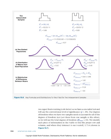
Figure 10.6 Key Formulas and Distributions for the t-Test for Two Independent Samples

(we expect brain-training to do better) so we have a one-tailed test and
will use the conventional level of significance ( = .05). Our degrees
p
of freedom when we have two samples needs to account for all of the
degrees of freedom (not just those from one sample or the other),
so we will use the total degrees of freedom (df Total = 23). We identify
each piece of information in the t-table to find the proper row and
column, and where they intersect is our t-cutoff, 1.714 (shown in
Figure 10.7).
356 S TATIS TI c S F OR L IFE

Copyright ©2024 Worth Publishers. Distributed by Worth Publishers. Not for redistribution.

11_statsresandlife1e_24717_ch10_343_389.indd 356 29/06/23 5:17 PM