Page 36 - 2023-bfw-Macro-Krugman-Econ-4e

Supply MODULE 1.5

In this Module, you will learn to:
• Draw a supply curve and interpret its meaning
• Define the law of supply and explain the relationship between the price of a
good or service and the quantity supplied
• Contrast the difference between movements along the supply curve with
changes in supply
• Explain the determinants of supply

The Supply Curve

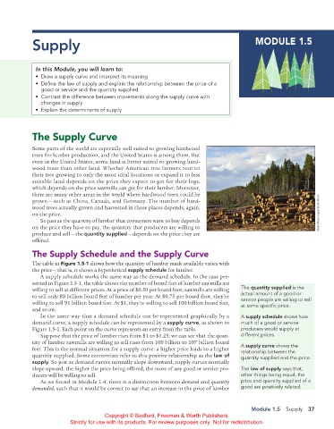
Some parts of the world are especially well suited to growing hardwood
trees for lumber production, and the United States is among them. But
even in the United States, some land is better suited to growing hard-
wood trees than other land. Whether American tree farmers restrict
their tree growing to only the most ideal locations or expand it to less
suitable land depends on the price they expect to get for their logs,
which depends on the price sawmills can get for their lumber. Moreover,
there are many other areas in the world where hardwood trees could be
grown — such as China, Canada, and Germany. The number of hard-
wood trees actually grown and harvested in those places depends, again,
on the price. Blink Photo/Alamy Stock Photo
So just as the quantity of lumber that consumers want to buy depends
on the price they have to pay, the quantity that producers are willing to
produce and sell — the quantity supplied — depends on the price they are
offered.

The Supply Schedule and the Supply Curve
The table in Figure 1.5-1 shows how the quantity of lumber made available varies with
the price — that is, it shows a hypothetical supply schedule for lumber.
A supply schedule works the same way as the demand schedule. In the case pre-
sented in Figure 1.5-1, the table shows the number of board feet of lumber sawmills are
willing to sell at different prices. At a price of $0.50 per board foot, sawmills are willing The quantity supplied is the
to sell only 80 billion board feet of lumber per year. At $0.75 per board foot, they’re actual amount of a good or
service people are willing to sell
willing to sell 91 billion board feet. At $1, they’re willing to sell 100 billion board feet, at some specific price.
and so on.
In the same way that a demand schedule can be represented graphically by a A supply schedule shows how
demand curve, a supply schedule can be represented by a supply curve, as shown in much of a good or service
Figure 1.5-1. Each point on the curve represents an entry from the table. producers would supply at
Suppose that the price of lumber rises from $1 to $1.25; we can see that the quan- different prices.
tity of lumber sawmills are willing to sell rises from 100 billion to 107 billion board A supply curve shows the
feet. This is the normal situation for a supply curve: a higher price leads to a higher relationship between the
quantity supplied. Some economists refer to this positive relationship as the law of quantity supplied and the price.
supply. So just as demand curves normally slope downward, supply curves normally
slope upward: the higher the price being offered, the more of any good or service pro- The law of supply says that,
ducers will be willing to sell. other things being equal, the
As we found in Module 1.4, there is a distinction between demand and quantity price and quantity supplied of a
demanded, such that it would be correct to say that an increase in the price of lumber good are positively related.

Module 1.5 Supply 37
Copyright © Bedford, Freeman & Worth Publishers.
Strictly for use with its products. For review purposes only. Not for redistribution.

02_APKrugman4e_40932_MacroU01_002_062.indd 37 05/07/22 10:51 AM