Page 52 - 2023-bfw-Macro-Krugman-Econ-4e

ModULE 1.6
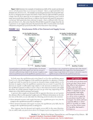
Figure 1.6-6 illustrates two examples of simultaneous shifts of the supply and demand
curves. In both panels there is an increase in demand — that is, a rightward shift of the
demand curve, from D to D — for example, representing an increase in the demand for lum-
2
1
ber due to changing tastes in home renovations. Notice that the rightward shift in panel (a)
is larger than the one in panel (b): we can suppose that panel (a) represents a year in which
many more people than usual choose to improve their homes and panel (b) represents a
normal year. Both panels also show a decrease in supply — that is, a leftward shift of the sup-
ply curve from S to S . Also notice that the leftward shift in panel (b) is larger than the one
1
2
in panel (a): we can suppose that panel (b) represents the effect of particularly severe beetle
infestations and panel (a) represents the effect of much less severe insect damage.
FIGURE 1.6-6 Simultaneous Shifts of the demand and Supply Curves

(a) One Possible Outcome: (b) Another Possible Outcome:
Price Rises, Quantity Rises Price Rises, Quantity Falls
Price Price
of Small of Large decrease S
lumber decrease S S lumber in supply 2
in supply 2 1
S 1
E 2 E
P 2 P 2 2

Small
E increase
E 1 P 1 in demand
P 1 1

D 2
D 1 D
Large increase D 2
in demand 1
Q 1 Q 2 Quantity of lumber Q 2 Q 1 Quantity of lumber

In panel (a) there is a simultaneous rightward shift of the demand panel (b) there is also a simultaneous rightward shift of the demand
curve and leftward shift of the supply curve. Here the increase in curve and leftward shift of the supply curve. Here the decrease in
demand is sufficiently large relative to the decrease in supply to cause supply is large enough relative to the increase in demand to cause the
both the equilibrium price and the equilibrium quantity to rise. In equilibrium price to fall while the equilibrium price rises.

In both cases, the equilibrium price rises from P to P as the equilibrium moves AP ECoN TIP
®
1
2
from E to E . But what happens to the equilibrium quantity, the quantity of lumber
1
2
bought and sold? In panel (a) the increase in demand is large enough relative to the To clarify what you know and
decrease in supply so that the equilibrium quantity rises as a result. In panel (b), the what you don’t know about
decrease in supply is sufficiently large relative to the increase in demand to cause the effect of simultaneous
the equilibrium quantity to fall as a result. That is, when demand increases and supply shifts, treat each shift
decreases, the actual quantity bought and sold can go either way, depending on the individually and identify the
relative sizes of the shifts in demand and supply. effect on equilibrium price
In general, when supply and demand shift in opposite directions, we can’t predict and quantity. Both shifts
the ultimate effect on the quantity bought and sold. Without information on the rela- will have the same effect
tive sizes of the shifts, we can only make the following prediction about the outcome: on either price or quantity,
so you know how that has
• • When demand increases and supply decreases, the equilibrium price rises, but the changed. The shifts will have
change in the equilibrium quantity is ambiguous. opposite effects on either
• • When demand decreases and supply increases, the equilibrium price falls, but the price or quantity, so unless
change in the equilibrium quantity is ambiguous. you know the relative sizes
of the shifts, that result is
Now suppose that the demand and supply curves shift in the same direction. ambiguous.
Can we safely make any predictions about the changes in price and quantity? In this

Module 1.6 Market Equilibrium, Disequilibrium, and Changes in Equilibrium 53
Copyright © Bedford, Freeman & Worth Publishers.
Strictly for use with its products. For review purposes only. Not for redistribution.

02_APKrugman4e_40932_MacroU01_002_062.indd 53 05/07/22 10:51 AM