Page 51 - 2023-bfw-Macro-Krugman-Econ-4e

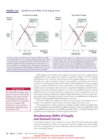
FIGURE 1.6-5 Equilibrium and Shifts of the Supply Curve

(a) Decrease in Supply (b) Increase in Supply
Price of Price of
lumber A decrease in lumber An increase in
supply . . . supply . . .
S 2 S 1 S 1 S 2

E 2 E 1
P 2 P 1
. . . leads to a . . . leads to a
Price movement along Price movement along
rises the demand curve to falls the demand curve to
a higher equilibrium a lower equilibrium
P 1 E 1 price and lower P 2 E 2 price and higher
equilibrium quantity. equilibrium quantity.

Demand Demand

Q s Q 2 Q 1 Quantity of Q 1 Q 2 Q s Quantity of
lumber lumber
Quantity falls Quantity rises

(a) Insect infestation in lumber-growing areas shifts the supply technology shifts the supply curve rightward from S to S creating
1
2,
curve leftward from S to S creating a shortage equal to (Q 1 −Q ) at a surplus equal to (Q s −Q ) at the original price, causing a decrease
s
2,
1
1
the original price, causing an increase in price and a decrease in in price and an increase in quantity supplied and a movement
quantity supplied and a movement along the demand curve. A along the demand curve. A new equilibrium is established at E ,
2
new equilibrium is established at E , where quantity demanded where quantity demanded again equals quantity supplied with a
2
equals quantity supplied with a higher equilibrium price, P , and lower equilibrium price, P , and a higher equilibrium quantity, Q .
2
2
2
a lower equilibrium quantity, Q . (b) The advance in sawmill
2
What happens to the market when supply increases? An increase in supply leads to
a rightward shift of the supply curve, as shown in panel (b) of Figure 1.6-5. The original
equilibrium is at E , the point of intersection of the original supply curve, S , and the
1
1
demand curve, with an equilibrium price P and equilibrium quantity Q . As a result of
1
1
an advance in technology, supply increases and S shifts rightward to S . At the original
1
2
price, P , a surplus of lumber now exists and the market is no longer in equilibrium. The
1
surplus causes a fall in price and an increase in quantity demanded, represented by a
®
AP ECoN TIP downward movement along the demand curve. The new equilibrium is at E , with an
2
A shift of the demand curve equilibrium price P and an equilibrium quantity Q . In the new equilibrium, E , the
2
2
2
does not cause a shift of the price is lower and the equilibrium quantity is higher than before. This can be stated as a
supply curve, and a shift of general principle: When supply of a good or service increases, the equilibrium price of the good or
the supply curve does not service falls, and the equilibrium quantity of the good or service rises.
cause a shift of the demand Note that a shift of the supply curve does not cause a shift of the demand curve. A
curve. A change in the change in the equilibrium price causes a movement along the demand curve.
equilibrium price causes a To summarize how a market responds to a change in supply: A decrease in supply leads to
movement along the curve a rise in the equilibrium price and a fall in the equilibrium quantity. An increase in supply leads to a fall
that didn’t shift. in the equilibrium price and a rise in the equilibrium quantity. That is, a change in supply causes
equilibrium price and quantity to move in opposite directions.
Simultaneous Shifts of Supply
and Demand Curves
It sometimes happens that simultaneous events shift both the demand and supply
curves at the same time. This is not unusual; in real life, supply curves and demand
curves for many goods and services shift quite often because the economic environ-
ment continually changes.
52 Macro • Unit 1 Basic Economic Concepts
Copyright © Bedford, Freeman & Worth Publishers.
Strictly for use with its products. For review purposes only. Not for redistribution.

02_APKrugman4e_40932_MacroU01_002_062.indd 52 05/07/22 10:51 AM