Page 29 - 2023-bfw-Macro-Krugman-Econ-4e

The table in Figure 1.4-2 shows two demand schedules. The first is a demand
schedule for 2020, the same one shown in Figure 1.4-1. The second is a demand
schedule for 2021. That demand schedule differs from the 2020 demand schedule
due to factors such as changing tastes for new homes and higher incomes, factors
that led to an increase in the quantity of lumber demanded at any given price. So at
each price, the 2021 schedule shows a larger quantity demanded than the 2020 sched-
ule. For example, the quantity of lumber consumers wanted to buy at a price of $1 per
board foot increased from 100 billion to 120 billion board feet per year, the quantity
demanded at $1.25 per board foot went from 89 billion to 107 billion board feet, and
so on.
What is clear from this example is that the changes that occurred between 2020
and 2021 generated a new demand schedule, one in which the quantity demanded
was greater at any given price than in the original demand schedule. The two curves
A change in demand is a shift in Figure 1.4-2 show the same information graphically. As you can see, the demand
of the demand curve, which schedule for 2021 corresponds to a new demand curve, D , that is to the right of the
2
changes the quantity demanded demand curve for 2020, D . This change in demand shows the increase in the quan-
at any given price. 1
tity demanded at any given price, represented by the shift in position of the original
A movement along the demand curve, D , to its new location at D .
1
2
demand curve is a change It’s crucial to make the distinction between such changes in demand and move-
in the quantity demanded of ments along the demand curve, which are changes in the quantity demanded
a good that is the result of a of a good that result from a change in that good’s price. Figure 1.4-3 illustrates the
change in that good’s price. difference.

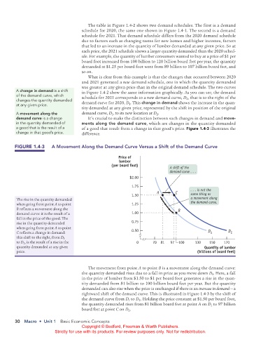
FIGURE 1.4-3 A Movement Along the demand Curve Versus a Shift of the demand Curve

Price of
lumber
(per board foot)
A shift of the
demand curve . . .
$2.00
1.75
. . . is not the
A C
1.50 same thing as
The rise in the quantity demanded a movement along
when going from point A to point 1.25 the demand curve.
B reflects a movement along the B
demand curve: it is the result of a 1.00
fall in the price of the good. The
rise in the quantity demanded 0.75
when going from point A to point
C reflects a change in demand: 0.50 D 1 D 2
this shift to the right, from D 1
to D 2 , is the result of a rise in the 0 70 81 97 100 130 150 170
quantity demanded at any given Quantity of lumber
price. (billions of board feet)

The movement from point A to point B is a movement along the demand curve:
the quantity demanded rises due to a fall in price as you move down D . Here, a fall
1
in the price of lumber from $1.50 to $1 per board foot generates a rise in the quan-
tity demanded from 81 billion to 100 billion board feet per year. But the quantity
demanded can also rise when the price is unchanged if there is an increase in demand — a
rightward shift of the demand curve. This is illustrated in Figure 1.4-3 by the shift of
the demand curve from D to D . Holding the price constant at $1.50 per board foot,
1
2
the quantity demanded rises from 81 billion board feet at point A on D to 97 billion
1
board feet at point C on D .
2
30 Macro • Unit 1 Basic Economic Concepts
Copyright © Bedford, Freeman & Worth Publishers.
Strictly for use with its products. For review purposes only. Not for redistribution.

02_APKrugman4e_40932_MacroU01_002_062.indd 30 05/07/22 10:50 AM