Page 12 - 2023-bfw-Macro-Krugman-Econ-4e

ModULE 1.2
the larger classroom worse off — by moving them to the room that
is too small.
Returning to our castaway example, as long as Alexis produces
a combination of coconuts and fish that is on the production pos-
sibilities curve, her production is efficient. No resources are being
wasted, so there is no way to make more of one good without mak-
ing less of the other. For example, at point A , the 15 coconuts she
gathers are the maximum quantity she can get given that she has
chosen to catch 20 fish. At point B , the 9 coconuts she gathers are
the maximum she can get given her choice to catch 28 fish. The
economy is producing efficiently if it is producing at any point on David Grossman/Alamy
its production possibilities curve.
Now suppose that for some reason Alexis is at point C , produc-
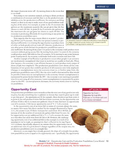
ing 20 fish and 9 coconuts. Then this one-person economy is pro- A crowded classroom reflects inefficiency if switching to
ducing inefficiently: it is missing the opportunity to produce more a larger classroom would make some students better
of either or both goods with no trade-off. Likewise, production at off without making anyone worse off.
any other point inside (below) the production possibilities curve is
also inefficient. By moving from point C to point A , the economy could produce more
coconuts without giving up any fish. By moving from point C to point B , the economy
could produce more fish with no loss of coconuts. Or by moving to any point between
point A and point B , the economy could make both more coconuts and more fish.
Another example of inefficiency in production occurs when people in an economy
are involuntarily unemployed: they want to work but are unable to find jobs. When
that happens, the economy is not efficient because it could produce more output if
those people were employed. The production possibilities curve shows all the com-
binations of two goods that could be produced if all resources were fully employed.
Changes in unemployment move the economy closer to, or further away from, the
production possibilities curve ( PPC ). But the curve itself is determined by what would
be possible if there were no unemployment in the economy. Greater unemployment is

represented by points farther below the PPC — the economy is not reaching its possibil-
ities if it is not using all of its resources. Lower unemployment is represented by points

closer to the PPC — as unemployment decreases, the economy moves closer to reaching
its possibilities.

Opportunity Cost AP ECoN TIP
®
The production possibilities curve reminds us that the true cost of any good is not only Opportunity Cost =
its price, but also everything else in addition to money that must be given up in order Opportunity Lost (the
to get that good — the opportunity cost . If, for example, Alexis decides to go from point A financial or nonfinancial cost
to point B , she will produce 8 more fish but 6 fewer coconuts. So the opportunity cost of a choice not taken)
of those 8 fish is the 6 coconuts not gathered. Since 8 extra fish have an opportunity
3

6
cost of 6 coconuts, 1 fish has an opportunity cost of ⁄8 = ⁄4 of a coconut.
Is the opportunity cost of an extra fish in terms of coconuts always the same,
no matter how many fish Alexis catches? In the example illustrated by Figure
no matter ho w man y f ish Alexis catches? In the ex am ple illustrated b y Figure
1.2-1 , the answer is yes. If Alexis increases her catch from 28 to 40 fish, an
1 .2-1 , the answ er is y es. If Alexis increases her catch from 28 to 40 f ish, an
increase of 12, the number of coconuts she gathers falls from 9 to zero. So
her opportunity cost per additional fish is ⁄12 = ⁄4 of a coconut, the same
3

9
as it was when her catch went from 20 fish to 28. However, the unchang-
ing opportunity cost of an additional fish in this example is a result of an
tion
that’s
p
ref
wa
y
Figure
the
lected

in
assum
w
e’v
p
tion
e
an
assumption we’ve made, an assumption that’s reflected in the way Figure
assum
made,
1.2-1 is drawn. Specifically, whenever we assume that the opportunity cost of
1 .2-1 is dra wn. Specif ically , whenev er w e assume that the oppor tunity cost of Creativ Studio Heinemann/Getty Images
an additional unit of a good doesn’t change regardless of the output mix, the
an additional unit of a good doesn’t change regar dless of the output mix, the
production possibilities curve is a straight line.
Moreover, as you might have already guessed, the slope of a straight-line produc-
Moreover, as you might have already guessed, the slope of a straight-line produc-
tion possibilities curve is equal to the opportunity cost — specifically, the opportunity
tion possibilities curve is equal to the opportunity cost — specifically, the opportunity
Module 1.2 Opportunity Cost and the Production Possibilities Curve Model 13
Copyright © Bedford, Freeman & Worth Publishers.
Strictly for use with its products. For review purposes only. Not for redistribution.
02_APKrugman4e_40932_MacroU01_002_062.indd 13 05/07/22 10:50 AM