Page 13 - 2023-bfw-Macro-Krugman-Econ-4e

cost for the good measured on the horizontal axis in terms of the good measured
on the vertical axis. In Figure 1.2-1, the production possibilities curve has a constant
slope of − ⁄4, implying that Alexis faces a constant opportunity cost per fish equal to ⁄4 of
3
3
a coconut. (A review of how to calculate the slope of a straight line is found in the
Appendix.) This is the simplest case, but the production possibilities curve model can
also be used to examine situations in which opportunity costs change as the mix of
output changes.
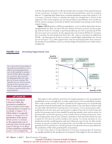
Figure 1.2-2 illustrates a different assumption, a case in which Alexis faces increas-
ing opportunity cost. Here, the more fish she catches, the more coconuts she has to give
up, and vice versa. For example, to go from producing zero fish to producing 20 fish,
she has to give up 5 coconuts. So the opportunity cost of those 20 fish is 5 coconuts.
But to increase her fish production from 20 to 40 — that is, to produce an additional
20 fish — she must give up 25 more coconuts, a much higher opportunity cost. As you
can see in Figure 1.2-2, when opportunity costs are increasing rather than constant,
the production possibilities curve is a concave-shaped (bowed-out) curve rather than a
straight line.

FIGURE 1.2-2 Increasing opportunity Cost

Quantity
of coconuts
Producing the rst . . . requires giving
35 20 sh . . . up 5 coconuts.
30 But producing 20
The concave (bowed-out) shape of more sh . . .
the production possibilities curve 25 A
reflects increasing opportunity
cost. In this example, to produce 20
the first 20 fish, Alexis must give . . . requires
up 5 coconuts. But to produce 15 giving up 25
an additional 20 fish, she must more coconuts.
give up 25 more coconuts. The 10
opportunity cost of fish increases
because as Alexis catches more 5
fish, she must make increasing use PPC
of resources specialized for coco- 0 10 20 30 40 50
nut production. Quantity of sh

®
AP ECoN TIP
Although it’s often useful to work with the simple assumption that the production
The use of specialized
resources makes the possibilities curve is a straight line, in reality, opportunity costs are typically increasing.
production possibilities When only a small amount of a good is produced, the opportunity cost of producing
curve concave to the origin, that good is relatively low because the economy needs to use only those resources that
meaning that it is bowed out are especially well suited for its production. For instance, if an economy grows only a
as shown in Figure 1.2-2. small amount of corn, that corn can be grown in places where the soil and climate are
When there is no speciali- perfect for growing corn but less suitable for growing another crop, such as wheat. So
zation of resources for the growing that corn involves giving up only a small amount of wheat production. Once
production of the goods, the economy grows a lot of corn, however, land that is well suited for wheat but isn’t
there can be no increase so great for corn must be used to produce corn anyway. As a result, increases in corn
in the opportunity cost of production involve sacrificing more and more wheat per unit of corn. In other words,
making more of either good, as more of a good is produced, its opportunity cost typically rises because resources
and no change in the slope specialized for the production of that good are used up and resources specialized for
of the production possibilities the production of the other good must be used instead.
curve — it is a straight line. In some cases, there is no specialization of resources, meaning that all resources
are equally suitable for the production of each good. That might be the case when the

14 Macro • Unit 1 Basic Economic Concepts
Copyright © Bedford, Freeman & Worth Publishers.
Strictly for use with its products. For review purposes only. Not for redistribution.

02_APKrugman4e_40932_MacroU01_002_062.indd 14 05/07/22 10:50 AM